How fine is fine

State-level data would be adequate, if the weather didn't play such a key role in our business. It is crucial to get as fine-grained data as possible, but without spending money for commercial licenses, this data is very hard to come by. Frugal as I am, I figured I would take a stab at it using a free dataset from the National Oceanic and Atmospheric Administration (NOAA) that measures historical monthly cooling degree days (how many days the daily mean temperature rises above 65 degrees Fahrenheit) across all the states, and try to squeeze out as much as I can from it.

Temperature gradient

The first, naive approach I had was to simply create a temperature gradient between the states. So if the CDD for state A was 300 CDD for a given month, and state B (let say it's directly adjacent) was 400 CDD for the same month, then we can just create a gradient between 300 and 400 for all the points between the two states.

This raises several questions. The first is how do you pick where to put the 300 in state A, is it the centroid of the state? The measure is presumably an aggregate, so do you locate all the measuring stations and calculate the centroid from those? No matter how you choose, it will be more or less arbitrary, but we will take steps later to account for that.

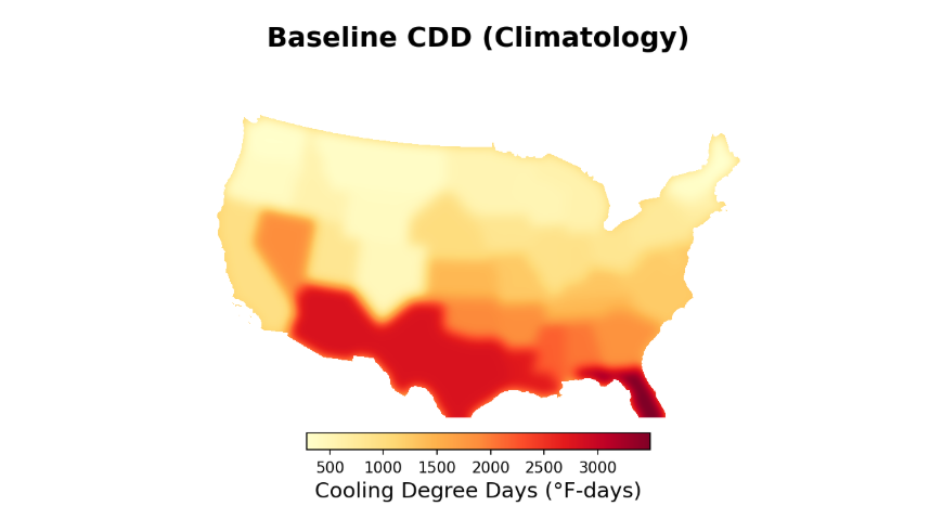
Next, what do we do about adjacency? Consider, for instance, Florida and Georgia in the above example. The high differential in CDD between the two states causes a steep gradient between them. While this is ok on a macro scale, on the country or zip level, this leads to highly inaccurate data.

So we see simple linear gradient between state centroids causes distortions and bias in measurements, but can we devise a better approach?

A naturally derived solution

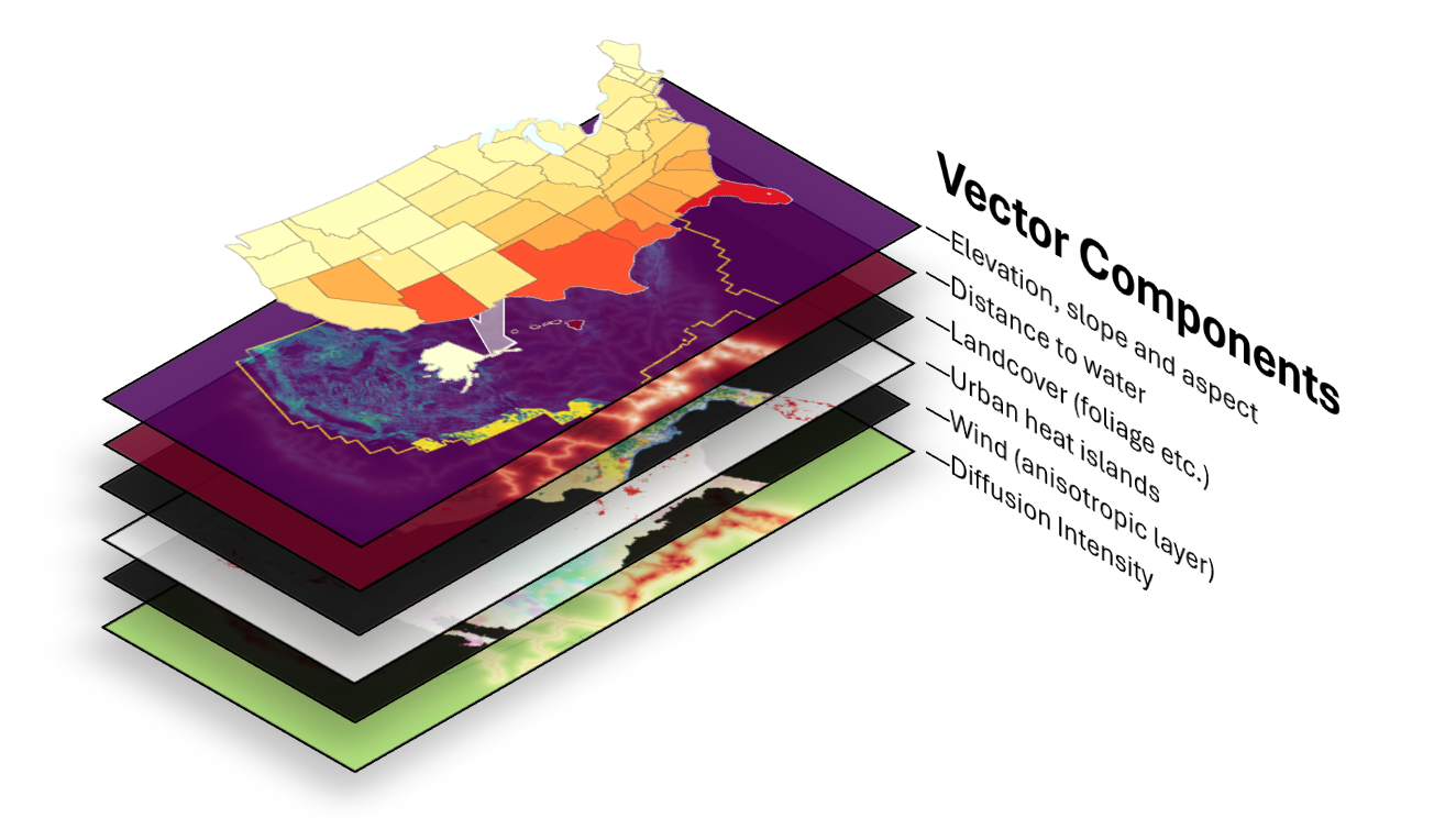
Let's take a step back and study how temperature actually behaves. It is deterministically influenced heavily by several natural features, such as the topology, water bodies and even urbanization. We can stack these into many layers that define how the temperature actually permeates the geography of each state.

The way I intuited this is by pouring paint on a map of the United States in each state, wherein the paint color represents the cooling degree days of the state. The fluidity of the paint causes it to spread from the center of the state and eventually mix slightly with the neighboring states, creating that smooth gradient we mentioned earlier. However, if, before we pour, we alter the topology and texture (macro and micro features) of the map, by raising or lower it accordingly, then the paint will flow through it at different rates. It will still mix with the neighboring paints, but it will be in a way consistent with how actual temperature propagates.

In practice

We can take a very similar approach ourselves. By building a field of influence vectors, we can change how that initial state-level CDD value gets propagated down to smaller regions. we start with all the vectors at the same length, which represents that perfectly smooth map. Then we adjust the length of each vector by stacking different physically representative layers, like the altitude, the distance to the nearest water, the brush or tree cover, and many other features. This effects the magnitude of the vectors, and which determines how the paint (CDDs) flows over it.

End-to-end workflow

• Start with state-level CDD forecast signals and historical climate baselines, then set up a common national grid so every dataset lines up geographically.
• Layer in physical drivers that shape local temperature behavior, including elevation, slope, distance to water, land cover, and urbanization effects.
• Convert those layers into a conductivity surface that controls how strongly heat anomalies can spread from one area to another.
• Seed each state with its starting anomaly signal, then diffuse that signal across the map so neighboring areas influence each other naturally instead of stopping at political borders.
• Keep state forecasts as soft anchors (guidance, not hard walls) so the final map stays realistic while still respecting the broader forecast direction.
• Recompose final local CDD values and aggregate to ZIP, county, and MSA outputs for downstream demand and replacement-rate forecasting.

How this drives forecasting decisions

The practical value of the model is that it turns a single state-level weather signal into local demand risk. Instead of saying "Texas is hot this year," we can identify which specific ZIPs and MSAs are likely to carry the highest cooling burden and therefore the highest pressure on installed HVAC systems.

At a planning level, this feeds directly into three decisions:

• Where to stage inventory and service capacity ahead of peak demand windows.
• Which regions are likely to see higher replacement activity versus routine service activity.
• How to prioritize sales, dealer support, and marketing spend by local opportunity rather than state averages.

In short, the output is not just a better weather map. It is a geographic demand signal that helps convert climate variability into concrete operational and commercial actions.